What you will learn in this lesson:
- The geometric intuition behind "the line that minimizes total squared vertical distance"
- Why we minimize squared error rather than raw error or absolute error
- A full worked numeric example computing slope and intercept by hand on five data points
- What residuals tell you about how well (or badly) a line fits
- Runnable code that fits a regression line and plots it against the data
Fitting a Line to Data
Simple linear regression is the most basic predictive model in machine learning, and it's the right place to start because nearly every idea you'll use later, loss functions, optimization, residual analysis, shows up here first in its simplest possible form.
The goal is to find the straight line that best describes the relationship between one input variable
x and one output variable y. A line is defined by two numbers: its slope m
(how steeply y increases as x increases) and its intercept b (the value of y when x is zero):
y = mx + b
For example, if you're predicting a house's price from its size in square meters, m tells you how
much the price increases for each additional square meter, and b is a baseline price offset. The
challenge: out of the infinitely many possible lines you could draw through a scatter of points, which one is
"best"?
The Geometric Picture: Minimizing Vertical Distance
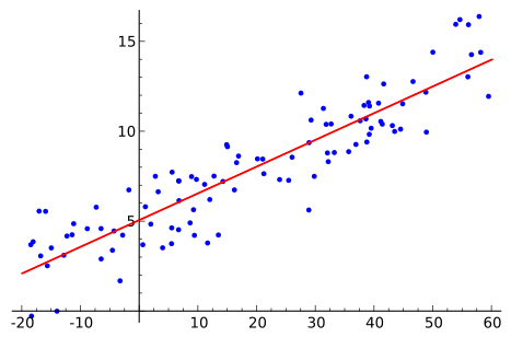
Picture your data as dots scattered on a graph. Any candidate line you draw through them will pass close to some points and far from others. For each point, draw a small vertical segment connecting the point straight up or down to the line. That segment's length is the residual (the error) for that point: the actual y-value minus the line's predicted y-value at that x.
"Best" needs a precise definition, and the geometric goal of least-squares linear regression is exactly this: find the line that minimizes the sum of the squared lengths of all those vertical segments. Not the sum of raw lengths. The sum of squared lengths.
Two things would go wrong if you used raw, unsquared residuals. First, positive residuals (points above the line) and negative residuals (points below the line) would cancel each other out when summed, so a line could have enormous total error in both directions and still report a deceptively small sum. Second, without squaring, the optimization problem doesn't have a single clean closed-form answer in the same way.
Squaring fixes the cancellation problem (every squared term is positive, so errors can never cancel) and has a second, important side effect: it penalizes large errors disproportionately more than small ones. A residual of 4 contributes 16 to the sum; a residual of 1 contributes only 1.
This means the least-squares line is pulled strongly away from leaving any single point very far off, even at the cost of fitting the bulk of the points slightly less perfectly. This is also precisely why least-squares regression is sensitive to outliers. One point far from the rest can have an outsized pull on where the line ends up, because its large residual gets squared.
There is a closed-form formula for the exact slope and intercept that minimize this sum. You never need to try every possible line by brute force. (There's also an iterative numerical method called gradient descent, useful when closed-form solutions aren't available, which you'll meet in later lessons.)
A Worked Numeric Example
Suppose you have five data points relating hours studied (x) to exam score (y):
| Hours Studied (x) | Exam Score (y) |
|---|---|
| 1 | 52 |
| 2 | 58 |
| 3 | 65 |
| 4 | 73 |
| 5 | 80 |
The mean of x is 3 and the mean of y is 65.6. The least-squares slope is the sum of
(x − mean_x)(y − mean_y) divided by the sum of (x − mean_x)². Working through each
point:
- x=1: (1−3)(52−65.6) = (−2)(−13.6) = 27.2, and (1−3)² = 4
- x=2: (2−3)(58−65.6) = (−1)(−7.6) = 7.6, and (2−3)² = 1
- x=3: (3−3)(65−65.6) = 0, and (3−3)² = 0
- x=4: (4−3)(73−65.6) = 7.4, and (4−3)² = 1
- x=5: (5−3)(80−65.6) = 28.8, and (5−3)² = 4
Summing the numerators gives 71.0, and summing the denominators gives 10. So the slope
m = 71.0 / 10 = 7.1. The intercept is b = mean_y − m × mean_x = 65.6 − 7.1 × 3 = 44.3.
The fitted line is y = 7.1x + 44.3: each extra hour of study is associated with roughly 7.1
additional points on the exam, and a student who studied zero hours would be predicted to score about 44.3.
Reading the Residuals
Once you have the line, plug each x back in and compare the prediction to the actual y:
| x | Actual y | Predicted y (7.1x + 44.3) | Residual (actual − predicted) |
|---|---|---|---|
| 1 | 52 | 51.4 | +0.6 |
| 2 | 58 | 58.5 | −0.5 |
| 3 | 65 | 65.6 | −0.6 |
| 4 | 73 | 72.7 | +0.3 |
| 5 | 80 | 79.8 | +0.2 |
The residuals here are small and have no obvious pattern. They don't consistently grow as x increases, and they don't form a curve. That's exactly what you want to see: it suggests a straight line is a genuinely good model for this relationship.
If instead the residuals had grown steadily larger for bigger x, or had formed a clear U-shape (negative, then positive, then negative again), that would be a strong signal that the true relationship isn't linear and a straight line is the wrong hypothesis space for this data, an idea you saw formally in the first lesson of this course.
Fitting and Plotting the Model in Python
In practice, you will almost never compute this by hand. scikit-learn's LinearRegression handles it
in a few lines, and matplotlib lets you see the fitted line against the actual data immediately:
import numpy as np
import matplotlib.pyplot as plt
from sklearn.linear_model import LinearRegression

# Hours studied and exam scores from the worked example above
X = np.array([[1], [2], [3], [4], [5]])  # sklearn expects a 2D array of features
y = np.array([52, 58, 65, 73, 80])

model = LinearRegression()
model.fit(X, y)

print("Slope:", model.coef_[0])        # ~7.1
print("Intercept:", model.intercept_)  # ~44.3

# Predict the score for someone who studied 6 hours
prediction = model.predict([[6]])
print("Predicted score for 6 hours:", prediction[0])

# Plot the data points and the fitted line together
x_line = np.linspace(0, 6, 100).reshape(-1, 1)
y_line = model.predict(x_line)

plt.scatter(X, y, color="steelblue", label="actual data", zorder=3)
plt.plot(x_line, y_line, color="indianred", label="fitted line")
plt.xlabel("Hours studied")
plt.ylabel("Exam score")
plt.legend()
show_plot()
Note that scikit-learn expects the feature input X as a two-dimensional array, even when there's
only one feature. This is because the same API needs to support multiple features at once, which is exactly
where we're headed in the next lesson.
Limits of a Single Straight Line
Simple linear regression assumes the relationship between x and y is genuinely linear, and that there's only one input variable worth considering. Real-world problems are rarely that clean: house prices depend on size, location, age, and dozens of other factors simultaneously, and many relationships curve rather than follow a straight line.
A common misconception is that a low residual sum in your training data automatically means the model is "correct." It only means the model fits a straight line as well as a straight line possibly can to that data, which says nothing about whether a straight line was the right hypothesis space to begin with. Simple linear regression is the foundation, but it's a starting point, not the final tool. The next lesson extends this same idea to handle multiple input features at once.
Least-squares regression minimizes squared residuals, not raw ones. That single choice is why the line is sensitive to outliers (a residual of 4 costs 16, not 4) and why positive and negative errors can't cancel each other out. Always check the residuals after fitting: a random scatter around zero means the line is a reasonable fit, while a curved or growing pattern in the residuals means the data wasn't linear to begin with, no matter how "good" the line looks on the scatter plot.