K-Nearest Neighbors Classification

What you will learn in this lesson:

• The core idea behind K-Nearest Neighbors classification, and why it's called a "lazy learner"
• How to choose K and the bias-variance tradeoffs involved
• Why feature scaling matters enormously for KNN specifically, with a runnable demonstration
• How distance metrics and the curse of dimensionality affect KNN
• How to fit a KNN classifier with scikit-learn

The Core Idea: Classify by Your Neighbors

K-Nearest Neighbors (KNN) is one of the simplest classification algorithms conceptually, and it works almost exactly the way it sounds. To classify a new data point, you look at the K training examples that are closest to it (using some distance measure, typically straight-line Euclidean distance), and you assign the new point whatever class is most common among those K neighbors. There's no explicit formula being fit, no coefficients being learned in advance, the entire "model" is just the stored training data plus a rule for measuring distance and voting.

This is why KNN is often called a "lazy learner" or "instance-based" method, there's no upfront training phase that builds an internal representation; all the actual work happens at prediction time, when the algorithm searches through the stored training points to find the nearest ones.

Compare this to something like linear regression, where all the heavy computation happens once, during fitting, and predicting on a new point is just plugging numbers into a formula. KNN inverts that: fitting is essentially free (just store the data), and every single prediction does real work.

For example, imagine classifying whether a new customer is likely to churn based on their account age and monthly spend. With K=5, you'd find the 5 existing customers whose account age and spend are most similar to the new customer, see how many of those 5 churned versus stayed, and predict whichever outcome is the majority among them. If 4 out of 5 of the nearest customers churned, you'd predict churn for the new customer too.

Choosing K: A Balancing Act

The single hyperparameter you need to choose for KNN is K, the number of neighbors to consult, and this choice directly controls where the model sits on the bias-variance spectrum from earlier in the course.

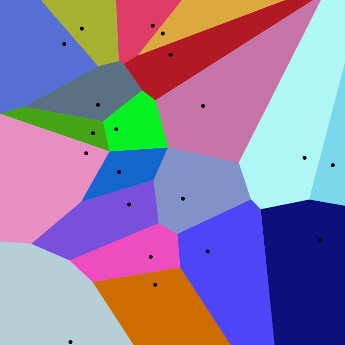
A very small K, such as K=1, means the prediction for any point depends entirely on its single closest neighbor. This makes the model extremely sensitive to noise: a single mislabeled or unusual training point can flip the prediction for any nearby new point.

The decision boundary becomes jagged and overfit to quirks in the training data (visually, it looks like a Voronoi diagram, a patchwork of irregular regions, one per training point), this is the high-variance, low-bias end of the spectrum.

A very large K, on the other hand, means each prediction is a vote across a large chunk of the dataset, which smooths out noise but can also wash out genuinely meaningful local patterns.

Taken to the extreme, if K equals the total number of training points, every prediction becomes the same: simply the most common class overall, regardless of where the new point actually sits. This is the high-bias, low-variance end of the spectrum, an oversmoothed model that ignores local structure entirely.

In practice, the right K is usually found through cross-validation: try a range of values (say, 1, 3, 5, 7, 11, 15, 21...) and pick whichever gives the best validation performance, typically measured by plotting validation accuracy against K and looking for where it peaks before degrading again. Odd numbers are common in binary classification to avoid tie votes, though scikit-learn breaks ties by ordering anyway if you do use an even K.

Why Feature Scaling Matters So Much

KNN's entire mechanism depends on measuring distance between points, which makes it far more sensitive to feature scale than most other algorithms in this course. Suppose you're predicting loan default risk using "annual income" (ranging from $20,000 to $200,000) and "credit utilization ratio" (ranging from 0 to 1).

Without scaling, the income feature's raw numeric range completely dominates the distance calculation, a $5,000 difference in income will swamp a 0.5 difference in credit utilization in the Euclidean distance formula, even if the utilization ratio is actually the far more predictive feature.

The fix is straightforward: standardize every feature (subtract the mean, divide by the standard deviation) before computing any distances, so that each feature contributes comparably to the distance regardless of its original units or range. Skipping this step is one of the most common beginner mistakes when applying KNN, and it can silently make an otherwise reasonable model perform far worse than it should, without throwing any error or warning to tell you something is wrong.

The example below makes this concrete: it trains the exact same KNN classifier on the exact same data, once without scaling and once with, and compares accuracy.

import numpy as np
from sklearn.neighbors import KNeighborsClassifier
from sklearn.preprocessing import StandardScaler
from sklearn.model_selection import train_test_split

np.random.seed(0)

# Features: [annual_income (large scale), credit_utilization (0-1 scale)]
# The true pattern: high utilization -> more likely to default, income is a weak secondary signal
n = 200
income = np.random.uniform(20000, 200000, n)
utilization = np.random.uniform(0, 1, n)
noise = np.random.randn(n) * 0.05
default_prob = utilization + noise
y = (default_prob > 0.5).astype(int)
X = np.column_stack([income, utilization])

X_train, X_test, y_train, y_test = train_test_split(X, y, test_size=0.3, random_state=0)

# Without scaling: income's huge numeric range dominates the distance calculation
knn_unscaled = KNeighborsClassifier(n_neighbors=5)
knn_unscaled.fit(X_train, y_train)
acc_unscaled = knn_unscaled.score(X_test, y_test)

# With scaling: both features contribute comparably to distance
scaler = StandardScaler()
X_train_scaled = scaler.fit_transform(X_train)
X_test_scaled = scaler.transform(X_test)
knn_scaled = KNeighborsClassifier(n_neighbors=5)
knn_scaled.fit(X_train_scaled, y_train)
acc_scaled = knn_scaled.score(X_test_scaled, y_test)

print("Accuracy WITHOUT scaling: {:.3f}".format(acc_unscaled))
print("Accuracy WITH scaling:    {:.3f}".format(acc_scaled))

Run this a few times with different random seeds, the scaled version should consistently match or beat the unscaled one, often by a wide margin, since the true underlying pattern here depends almost entirely on utilization, a feature that gets nearly drowned out by income's scale when distances are computed on raw, unscaled values.

Distance Metrics and the Curse of Dimensionality

Euclidean distance is the default in scikit-learn's KNeighborsClassifier, but it isn't the only option, and the choice can matter. Manhattan distance (sum of absolute coordinate differences) is sometimes preferred for high-dimensional or grid-like data, and is less sensitive to any single feature having an extreme outlier value, since differences aren't squared. For categorical or binary features, specialized distance metrics like Hamming distance are often more appropriate than treating one-hot encoded columns as ordinary continuous numbers.

A more fundamental issue is the curse of dimensionality: as the number of features grows, the notion of "nearest neighbor" starts to break down. In high-dimensional spaces, data points tend to spread out so much that the distance between the closest and farthest neighbor becomes nearly the same, the very notion of "near" loses its meaning.

This is a genuine limitation of KNN (and any purely distance-based method) on high-dimensional data, and it's one reason KNN tends to work best on datasets with a modest number of well-chosen, meaningfully scaled features, rather than hundreds of raw columns.

Practical Notes

KNN is a great starting point for understanding distance-based methods, but keep in mind it can become slow on very large datasets, since (in its naive form) every prediction requires scanning the stored training data to find nearest neighbors, an O(n) operation per prediction.

In practice, libraries like scikit-learn use smarter data structures (KD-trees or ball trees) to speed this up substantially for lower-dimensional data, though these speedups degrade as dimensionality grows, another manifestation of the curse of dimensionality above. For very large or very high-dimensional datasets, approximate nearest-neighbor libraries or a switch to a parametric model entirely is often the more practical choice.