What you will learn in this lesson:
- Mean, median, variance, and standard deviation, with a full worked numeric example
- What a probability distribution is, and why the normal distribution shows up everywhere (the Central Limit Theorem, briefly)
- The bias-variance tradeoff explained with concrete numbers, not just an analogy
- How bias and variance map directly onto underfitting and overfitting, the idea you'll meet formally in a later lesson
- Runnable code to compute these statistics and visualize a normal distribution yourself
Mean, Median, Variance, and Standard Deviation, Worked by Hand
Before fitting any model, you need a vocabulary for describing data. Let's use one concrete dataset throughout this section: the ages of 7 customers in a sample: 22, 25, 25, 30, 35, 40, 95.
The mean is the sum divided by the count: (22+25+25+30+35+40+95) / 7 = 272 / 7 ≈ 38.86. Notice that one outlier (95) pulled the mean well above where most of the data actually sits.
The median is the middle value once sorted: 22, 25, 25, 30, 35, 40, 95. The median is 30. The median ignored the outlier entirely and gives a much better sense of the "typical" customer age. This is exactly why median household income, not mean income, is the standard figure reported in economic statistics: a handful of billionaires would otherwise distort the picture for everyone else.
Variance measures spread around the mean. You take each value's distance from the mean, square it, and average those squared distances. Using our data (mean ≈ 38.86):
| Value | Deviation from mean | Squared deviation |
|---|---|---|
| 22 | -16.86 | 284.3 |
| 25 | -13.86 | 192.1 |
| 25 | -13.86 | 192.1 |
| 30 | -8.86 | 78.5 |
| 35 | -3.86 | 14.9 |
| 40 | 1.14 | 1.3 |
| 95 | 56.14 | 3151.7 |
Summing the squared deviations gives roughly 3914.9, and dividing by 7 gives a variance of about 559.3. Squaring matters for the same reason it matters for error metrics later in this course: it stops positive and negative deviations from canceling out, and it weights large deviations (like that 95) far more heavily than small ones. Notice how the outlier alone contributed over 80% of the total squared deviation.
Standard deviation is the square root of variance: √559.3 ≈ 23.65. Taking the square root brings the measure back into the original units (years, in this case), which is far easier to interpret than variance. Saying "the standard deviation of age is about 23.65 years" is meaningful in a way that "the variance is 559.3 squared-years" is not.
import numpy as np

ages = np.array([22, 25, 25, 30, 35, 40, 95])

print("Mean:", ages.mean())
print("Median:", np.median(ages))
print("Variance:", ages.var())
print("Standard deviation:", ages.std())

# Drop the outlier and see how much the mean moves vs the median
ages_no_outlier = np.array([22, 25, 25, 30, 35, 40])
print("\nWithout the 95-year-old outlier:")
print("Mean:", ages_no_outlier.mean())
print("Median:", np.median(ages_no_outlier))
What a Probability Distribution Is
A probability distribution describes how likely different outcomes are. Instead of a single summary number, you look at the full shape of how values are spread across a range of possibilities. For every possible value (or range of values), the distribution tells you how much probability "mass" sits there.
The Normal Distribution
The most famous distribution in statistics is the normal distribution (also called the Gaussian or "bell curve"). It is fully defined by just two numbers: its mean (where the peak sits) and its standard deviation (how wide or narrow the bell is). Its probability density function is:
f(x) = (1 / (σ√(2π))) · e^(−(x−μ)² / (2σ²))
where μ (mu) is the mean and σ (sigma) is the standard deviation. You rarely need to evaluate this formula by hand, but its shape matters: it's symmetric around μ, and the exponent's negative-squared-distance term is exactly why values far from the mean become exponentially rarer rather than just linearly rarer.
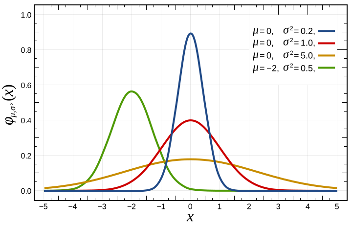
Concretely, suppose adult heights in a population follow a normal distribution with mean 170cm and standard deviation 8cm. The "68-95-99.7 rule" tells you: about 68% of people fall within one standard deviation of the mean (162cm to 178cm), about 95% fall within two standard deviations (154cm to 186cm), and essentially everyone (99.7%) falls within three (146cm to 194cm). Two numbers let you reason about an entire population without listing every individual measurement.
Why the Normal Distribution Shows Up Everywhere: the Central Limit Theorem
It's not a coincidence that so many real-world quantities are approximately normal. The Central Limit Theorem (CLT) says that when you add up (or average) many small, independent random effects, the result tends toward a normal distribution, regardless of the shape of the individual effects being summed.
A person's height is the cumulative result of many genetic and environmental factors, each contributing a small push up or down. Measurement error is the sum of many tiny independent sources of noise. Even the average of repeated dice rolls converges toward a bell shape as you average more rolls, even though a single die roll is uniformly distributed, not bell-shaped at all.
This is why the normal distribution is the default assumption in so many statistical methods: it's the distribution that "many small independent things added together" naturally converge to.
This matters directly for machine learning: many algorithms make implicit or explicit assumptions about how your data or your errors are distributed, and many evaluation techniques (confidence intervals, hypothesis tests, some forms of regularization derivation) rely on approximate normality to be mathematically justified.
import numpy as np
import matplotlib.pyplot as plt

# Simulate the Central Limit Theorem: average many rolls of a single die
# A single die roll is uniform (flat), not bell-shaped at all
np.random.seed(0)
single_rolls = np.random.randint(1, 7, size=10000)

# Now average groups of 10 rolls together, repeated 10000 times
averaged_rolls = np.random.randint(1, 7, size=(10000, 10)).mean(axis=1)

fig, axes = plt.subplots(1, 2, figsize=(10, 4))
axes[0].hist(single_rolls, bins=6, color="steelblue", edgecolor="white")
axes[0].set_title("Single die roll (uniform)")
axes[1].hist(averaged_rolls, bins=30, color="indianred", edgecolor="white")
axes[1].set_title("Average of 10 rolls (already bell-shaped)")
plt.tight_layout()
show_plot()
The Bias-Variance Tradeoff, With Real Numbers
Perhaps the single most important conceptual idea you will carry through the rest of this course is the bias-variance tradeoff. It explains why models fail, in one of exactly two distinguishable ways.
Picture this concretely: suppose the true relationship you're trying to learn is a gentle curve, but you only ever have 20 noisy data points sampled from it, and you repeat the experiment 100 times (100 different random samples of 20 points each), fitting a fresh model each time. Now look at the predictions all 100 models make for one specific input value, say x = 5:
- Low bias, low variance: the 100 predictions cluster tightly around the true value at x = 5. This is the model you want: accurate and consistent.
- Low bias, high variance: the 100 predictions average out to roughly the true value, but individually they're scattered all over the place. One sample's model says 4.2, another says 7.8, another says 5.9. The model is right "on average across many retrainings" but wildly inconsistent on any single training run. This is what overfitting looks like: an overly flexible model that latches onto the specific noise in whichever 20 points it happened to see.
- High bias, low variance: all 100 predictions land tightly clustered together, but consistently 2 units away from the true value, every single time. The model is consistent but systematically wrong. This is what underfitting looks like: a model too rigid to capture the true curve no matter what data it sees.
- High bias, high variance: predictions are both scattered and centered away from the truth, the worst of both worlds.
In modeling terms, bias is the error from a model being too simple (too constrained a hypothesis space, in the language of the previous lesson) to capture the true pattern. It makes systematic, repeatable mistakes no matter how much data you give it. Variance is the error from a model being too sensitive to the specific quirks of whichever training sample it happened to see. Retrain it on a slightly different sample and you get a noticeably different model.
The "tradeoff" is what makes this genuinely hard. Reducing bias, by making a model more flexible (adding features, increasing polynomial degree, growing a deeper tree), tends to increase variance, because a more flexible model has more freedom to fit noise.
Reducing variance, by simplifying the model, adding regularization, or using less flexible algorithms, tends to increase bias, because you've taken away some of the model's ability to fit genuine signal along with the noise. There is rarely a free lunch. The practical skill of machine learning is finding the sweet spot for your specific problem and dataset size.
import numpy as np
import matplotlib.pyplot as plt

# Demonstrate bias-variance with polynomial fits of different flexibility
np.random.seed(1)

def true_function(x):
    return np.sin(x)

x_plot = np.linspace(0, 6, 200)

fig, axes = plt.subplots(1, 2, figsize=(11, 4.5))

for degree, ax, title in [(1, axes[0], "Degree 1 (high bias, low variance)"),
                            (12, axes[1], "Degree 12 (low bias, high variance)")]:
    ax.plot(x_plot, true_function(x_plot), "k--", label="true function", linewidth=1)
    # Fit on 8 different random small samples to see how much the fitted curve swings
    for i in range(8):
        x_sample = np.random.uniform(0, 6, 12)
        y_sample = true_function(x_sample) + np.random.randn(12) * 0.2
        coeffs = np.polyfit(x_sample, y_sample, degree)
        ax.plot(x_plot, np.polyval(coeffs, x_plot), alpha=0.5, linewidth=1)
    ax.set_title(title)
    ax.set_ylim(-2, 2)

plt.tight_layout()
show_plot()
Run this and notice: the degree-1 (straight line) fits are nearly identical to each other every time, low variance, but none of them can bend to match the true sine curve, high bias. The degree-12 fits swing wildly from one random sample to the next, high variance, chasing the specific noise in whichever 12 points they saw.
Why This Matters for Everything Ahead
Every model in this course, from a simple straight-line regression to regularized multi-feature models, can be understood through this same lens. A plain linear regression is often high-bias (it can only draw straight lines, so it underfits curved relationships) but low-variance (it doesn't swing wildly between different training samples). A model with many unconstrained features and no regularization tends toward the opposite: low-bias (it can fit almost any pattern in the training set) but high-variance (a slightly different training set produces noticeably different coefficients).
Nearly every technique from here forward, regularization, feature scaling, cross-validation, and eventually ensembling, exists specifically to manage this tradeoff deliberately rather than stumbling into it by accident. Keep these worked numbers and the polynomial-fit picture in mind. We will come back to this exact tradeoff by name in the regularization lessons ahead, where ridge and lasso penalties are, quite literally, a dial for trading bias against variance.
Bias means systematically wrong: the model is too simple to capture the pattern. Variance means inconsistent across different training samples: the model is too flexible and latches onto noise. You cannot minimize both at once. Every modeling decision from here on (regularization strength, tree depth, K in KNN, number of trees) is really a dial that trades one for the other. When something underperforms, the first diagnostic question is always "is this bias or variance?", and the fix is different for each.