R² Explained: The Complete Beginner's Guide
What you will learn in this article:
- What R-squared (R²) measures and how to read it intuitively.
- Where R² comes from, specifically, how total variance is decomposed into explained and unexplained parts.
- Why R² can go below zero and what that signals about your model.
- When to use Adjusted R² instead of plain R², and why the distinction matters.
- The most common ways practitioners misuse R² and how to avoid them.
Introduction
Suppose you have trained a regression model and computed an RMSE of $14,830. Is that good or bad? Without context, it is genuinely difficult to say. If the house prices in your dataset range from $200,000 to $600,000, an average error of $14,830 might be quite acceptable. But if all prices cluster tightly between $200,000 and $210,000, that same RMSE would be a disaster. RMSE is powerful but it is anchored to the scale of the target variable, which makes it hard to compare across different problems.
R², the coefficient of determination, solves this problem by providing a scale-free, intuitive measure of model fit. Instead of asking how large the errors are in absolute terms, R² asks: what fraction of the total variation in the data does the model actually explain? An R² of 0.97 means the model captures 97 percent of the variation in the target variable, and that statement is equally meaningful regardless of whether you are predicting house prices in dollars or temperatures in Celsius.
Problem Statement
Every target variable has natural variation. House prices differ from one another; temperatures vary across days. Some of that variation can be explained by the features your model uses: bigger houses cost more, warmer months are hotter. But some variation remains unexplained, things your model does not capture.
The challenge for any evaluation metric is to express how much of the naturally occurring variation the model accounts for, in a way that does not depend on the specific scale or units of measurement. A metric that does this well lets you say things like "this model for predicting rainfall is better calibrated than this model for predicting house prices" even though the two targets are measured in completely different units and at completely different magnitudes.
Core Concepts and Terminology
| Term | Plain-language meaning |
|---|---|
| Variance | How spread out the actual values are. High variance means the target values differ a lot from one another. |
| SST (Total Sum of Squares) | The total amount of variation in the target variable, measured as how far each actual value is from the overall mean. |
| SSR (Residual Sum of Squares) | The variation the model fails to explain, measured as how far each actual value is from the model's prediction for it. Note: this post uses SSR to mean Residual Sum of Squares (unexplained error). Some sources use SSR for Sum of Squares due to Regression (the explained part). To avoid confusion, the unexplained portion is also called RSS in other references. |
| R² | The proportion of SST that the model explains. Ranges from 0 (no better than guessing the mean) to 1 (perfect fit). |
| Adjusted R² | A corrected version of R² that penalizes adding unnecessary predictors to the model. |
How It Works
To understand R², imagine the simplest possible prediction strategy: always predict the average value of the target. If house prices average $430,000, every house gets a predicted price of $430,000. This naive model captures zero information from the features, yet it will not be completely random either. It represents the floor, a baseline against which any real model should be measured.
The total variation in the data is measured by looking at how far each actual value is from that overall average. If prices range widely, there is a lot of total variation to explain. This total variation is called SST, the Total Sum of Squares. It is computed by taking the difference between each actual value and the mean, squaring those differences so that positive and negative deviations do not cancel, and summing them all up.
The model's predictions, if they are any good, should bring the predictions closer to the actual values than the mean alone did. The remaining unexplained error is measured by SSR, the Residual Sum of Squares: for each data point, how far is the actual value from the model's prediction?
R² is the fraction of SST that the model eliminates. Concretely: if SST is 53,000 and SSR is 1,100, then the model eliminated the vast majority of the variation, and R² equals 1 minus (1,100 divided by 53,000), which comes out to approximately 0.979. In plain terms: the model explains about 97.9 percent of the variation in the target.

Practical Example
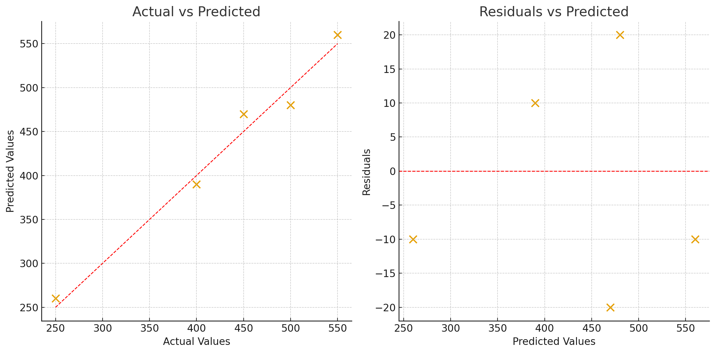
Consider a model predicting house prices for five properties. The actual prices, predicted prices, and the mean actual price are used to compute R².
| House | Actual Price (y) | Predicted Price (y-hat) | Deviation from mean (y - mean) | Residual (y - y-hat) |
|---|---|---|---|---|
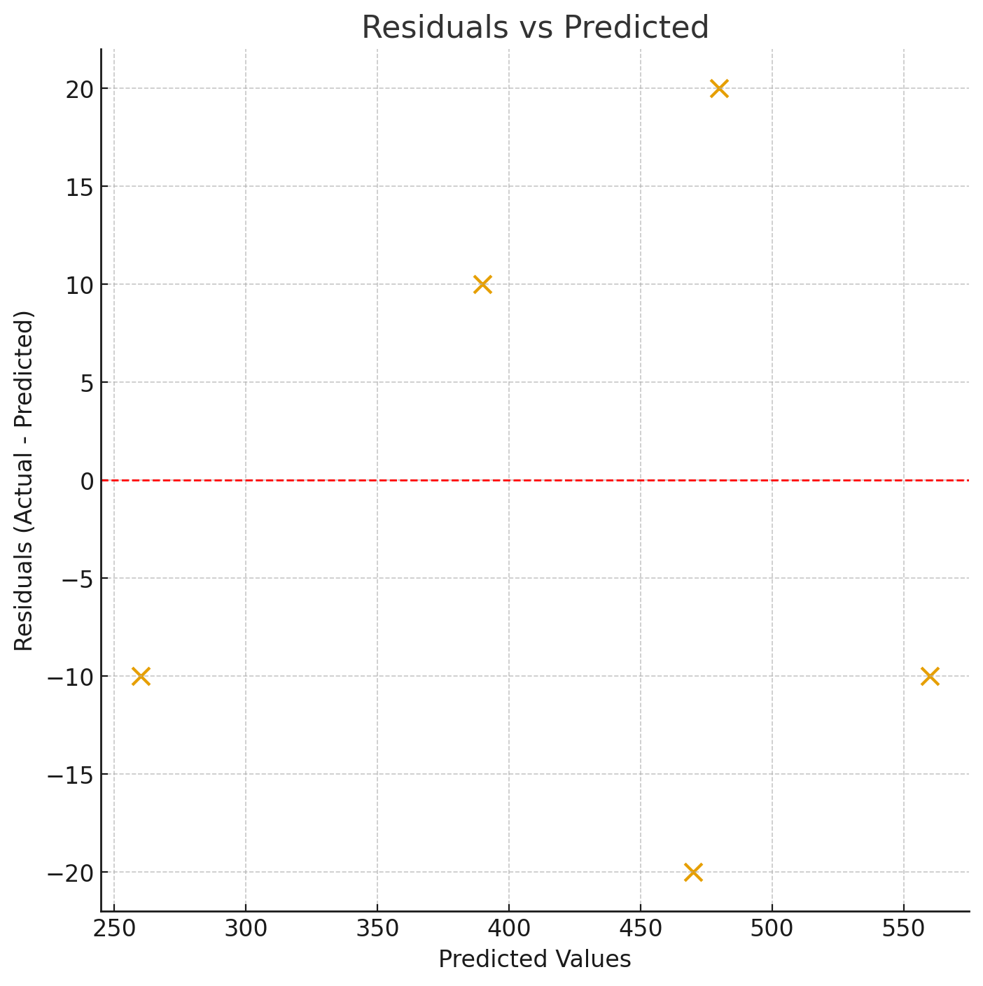
| 1 | 250 | 260 | −180 | −10 |
| 2 | 400 | 390 | −30 | +10 |
| 3 | 450 | 470 | +20 | −20 |
| 4 | 500 | 480 | +70 | +20 |
| 5 | 550 | 560 | +120 | −10 |
The mean actual price is 430. The SST, which sums the squared deviations from 430, comes out to 53,000. This represents how much total variation there is in house prices for these five cases.
The SSR, which sums the squared residuals, comes out to 1,100. This is the variation the model failed to explain.
R² is then 1 minus (1,100 divided by 53,000), which equals approximately 0.979. The model explains 97.9 percent of the price variation. Only about 2.1 percent remains unexplained. For a simple model on a small dataset, that is an excellent result.
Advantages
- Scale-free and universally interpretable. R² is always expressed as a proportion between 0 and 1 (or below 0 in extreme cases). This allows meaningful comparison across different domains and different scales of measurement, which pure error metrics like RMSE cannot offer.
- Intuitive communication with non-technical audiences. Saying "the model explains 97 percent of the variation in house prices" is immediately understandable to a business stakeholder who has no knowledge of statistics. It conveys model quality without requiring explanation of units or formulas.
- Connected to fundamental statistical theory. R² arises naturally from the decomposition of variance, which is a central idea in regression analysis. Understanding it unlocks deeper understanding of how regression models work and why they are evaluated the way they are.
Limitations and Trade-offs
- R² always increases when you add more predictors. Even if a new feature is completely useless noise, adding it to a linear regression model will never decrease R², and will usually increase it slightly. This creates a serious trap: a model with many irrelevant features can look excellent by R² while being genuinely overfit. This is precisely why Adjusted R² was invented.
- R² can go below zero. This happens when the model's predictions scatter more than the actual data does around its own mean. In other words, the model is performing worse than the naive strategy of always predicting the mean. This is always a sign of a serious problem.
- High R² does not mean the model is correct. A model can have a high R² while still being systematically biased, or while missing an obvious non-linear pattern in the data. Residual plots can reveal problems that R² hides entirely.
- Unreliable on small datasets and for non-linear data. With few observations, R² tends to be artificially inflated. On non-linear data, a linear model may have a low R² even when the underlying relationship is strong, simply because the model form is wrong.
Common Mistakes
- Comparing R² across models with different numbers of features without using Adjusted R². Adding features always increases or maintains plain R², so using it to compare models of different complexity systematically favors more complex models. Always use Adjusted R² in those comparisons.
- Treating a high R² as proof of a good model. R² measures how well a model fits the training data. A high training R² can coexist with poor generalization, especially in small datasets. Always evaluate on a held-out test set.
- Ignoring residual plots. R² summarizes overall variance explanation but cannot tell you whether the model is wrong in specific, systematic ways. Always examine residual plots alongside R².
- Using R² for classification or time-series models. R² is designed for regression. Applied naively to other model types, it can be misleading or even meaningless.
Best Practices
- Always report R² alongside RMSE or MAE. R² tells you how much variance is explained; RMSE tells you the actual magnitude of errors in real units. You need both.
- Use Adjusted R² when comparing models with different numbers of predictors. It penalizes unnecessary complexity and gives a fairer comparison.
- Evaluate R² on a held-out test set, not the training set. Training R² can be misleadingly high due to overfitting.
- Always inspect a residual plot. A high R² with a patterned residual plot is a warning sign that the model form is wrong.
- When communicating with non-technical stakeholders, convert R² to a percentage: R² of 0.87 becomes "the model explains 87 percent of the variation in the target."
Comparison with Related Metrics
| Metric | What it measures | Range | Units | Best used for |
|---|---|---|---|---|
| R² | Proportion of variance explained by the model | (-inf, 1] | Unitless | Scale-free comparison of fit quality |
| Adjusted R² | R² corrected for number of predictors | (-inf, 1] | Unitless | Comparing models with different numbers of features |
| RMSE | Typical prediction error magnitude | [0, inf) | Same as target | Communicating error in real-world terms |
| MAE | Average absolute prediction error | [0, inf) | Same as target | Interpretable error without outlier sensitivity |
FAQ
Why can R² be negative?
R² goes negative when the model's residuals are more dispersed than the actual data is around its own mean. Essentially, the model's predictions are worse than the trivial strategy of always predicting the average value. This is a red flag and usually indicates a deeply misspecified model, or predictions being applied to a distribution completely different from the training data.
What is a "good" R²?
It entirely depends on the domain. In tightly controlled physics experiments, R² values above 0.99 are expected. In social science models predicting human behaviour, an R² of 0.3 might be considered strong. The key is always to compare against a sensible baseline, and to ask whether the explained variation is sufficient for the intended use case.
Why does adding more predictors always increase R²?
In linear regression, adding any predictor, even one that is pure random noise, gives the model an extra degree of freedom to fit the training data. The model can always find at least a tiny way to use the new variable to reduce the sum of squared residuals, even if just by chance. Adjusted R² corrects for this by introducing a penalty that increases with the number of predictors.
Do I need both R² and RMSE?
Yes. R² is unitless and tells you how much variance is explained, but it does not tell you how large the errors are in real terms. RMSE gives you error magnitude in the actual units of the target variable. A model can have a high R² and still produce errors that are too large for practical use if the total variance in the target is very large. Always report both.
Can R² be used for non-linear models?
It can be computed, but its interpretation becomes more nuanced. For non-linear models, R² from the training set is especially unreliable as a goodness-of-fit measure, and the theoretical connection to variance decomposition weakens. Always pair it with residual diagnostics and evaluate on held-out data.
References
- James, G., Witten, D., Hastie, T., & Tibshirani, R. (2021). An Introduction to Statistical Learning (2nd ed.). Springer. [Book link]
- Chicco, D., Warrens, M. J., & Jurman, G. (2021). The coefficient of determination R². Biometrics, 77(2), 781–791. [DOI]
- Scikit-learn documentation: r2_score
- Wikipedia: Coefficient of Determination
Key Takeaways
- R² measures the proportion of variance in the target variable that the model explains, expressed on a 0-to-1 scale (or below zero for very poor models).
- An R² of 0 means the model is no better than always predicting the mean; an R² of 1 means perfect fit.
- R² can go below zero when the model performs worse than the trivial baseline of always guessing the mean, always a serious warning sign.
- Plain R² always increases or stays the same when you add more predictors, even useless ones. Use Adjusted R² when comparing models with different numbers of features.
- A high R² does not guarantee a correct model. Residual plots can reveal systematic biases that R² completely hides.
- Always evaluate R² on held-out test data and pair it with RMSE or MAE for a complete picture of model quality.
Related Articles