A Beginner's Guide to Elastic Net Regression (L1 + L2 Regularization)
1. Introduction: The Problem Elastic Net Solves
In the previous posts, we learned that Ridge shrinks all coefficients without removing any features, and Lasso can remove features by setting coefficients to exactly zero. Both are useful, but each has a specific weakness:
- Ridge keeps all features, it cannot remove truly irrelevant predictors.
- Lasso removes features, but behaves unpredictably when predictors are highly correlated. With two correlated features, Lasso tends to arbitrarily pick one and discard the other, even if both carry useful information.
Elastic Net solves both problems at once by combining the Ridge (L2) and Lasso (L1) penalties. It keeps Lasso's ability to set coefficients to zero (feature selection) while using Ridge's stability to handle correlated predictors gracefully, selecting groups of correlated features together rather than picking one arbitrarily.
2. The Elastic Net Penalty
Elastic Net adds both an L1 and an L2 term to the standard OLS loss function:
\[ J_{EN}(\beta) = \sum_{i=1}^n (y_i - \hat y_i)^2 + \alpha\left[(1-\rho)\tfrac{1}{2}\sum_{j=1}^p \beta_j^2 + \rho\sum_{j=1}^p |\beta_j|\right] \]
Two hyperparameters control the penalty:
-
\(\alpha\) (called
alphain scikit-learn), controls the overall strength of regularization. Larger \(\alpha\) = more shrinkage and more sparsity. \(\alpha = 0\) means no regularization (plain OLS). -
\(\rho\) (called
l1_ratioin scikit-learn), controls the mix between Ridge and Lasso. Ranges from 0 to 1:- \(\rho = 0\): pure Ridge (no feature selection)
- \(\rho = 1\): pure Lasso (maximum feature selection)
- \(\rho = 0.5\): equal blend of both
You can express this more compactly. The penalty term alone is:
\[ \text{Penalty} = \alpha\left[(1-\rho)\tfrac{1}{2}\|\beta\|_2^2 + \rho\|\beta\|_1\right] \]
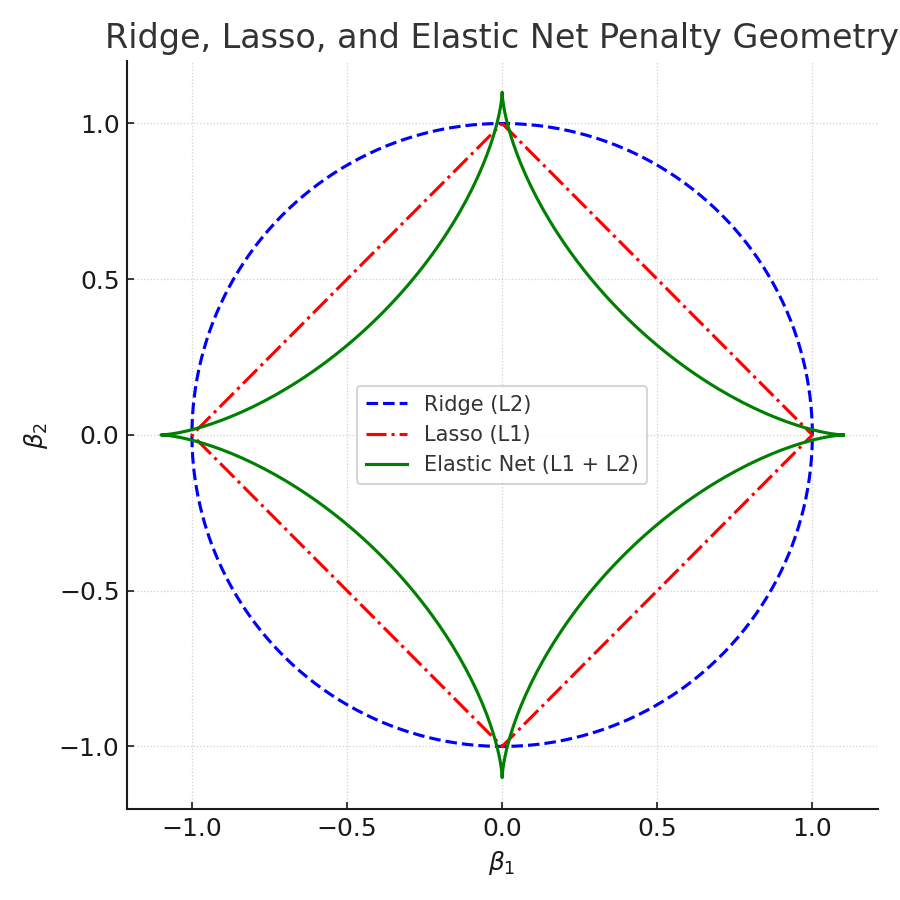
3. Geometric Intuition
Recall from the previous posts: Ridge uses a circular constraint region, and Lasso uses a diamond-shaped constraint region. The diamond's sharp corners are what force Lasso coefficients to zero.
Elastic Net's constraint region is a "rounded diamond", it sits between the circle and the diamond. It:
- Retains corners (so some coefficients can still be forced to zero, like Lasso).
- Has smooth edges (so correlated predictors tend to enter the model together, like Ridge).

4. How Elastic Net Updates Coefficients (Coordinate Descent)
Because the L1 penalty is not differentiable at zero, Elastic Net cannot be solved in closed form the way OLS can. Instead, it is typically optimized using coordinate descent: updating one coefficient at a time while holding all others fixed, cycling through all coefficients until convergence.
The update rule for each coefficient combines soft-thresholding (the Lasso component) with an L2 shrinkage factor (the Ridge component):
\[ \beta_j \leftarrow \frac{1}{1+\alpha(1-\rho)} \; S\!\left( \frac{1}{n}\sum_{i=1}^n x_{ij}(y_i - \hat y_{-j}),\; \frac{\alpha\rho}{n} \right) \]
Breaking this down:
- The inner part \(\frac{1}{n}\sum x_{ij}(y_i - \hat y_{-j})\) is the partial correlation between feature \(j\) and the residuals after removing feature \(j\)'s contribution, call it \(z\).
- Soft-thresholding \(S(z, \gamma)\): if \(|z| < \gamma\), the coefficient is set to zero (Lasso feature selection). Otherwise, \(z\) is shrunk by \(\gamma\).
- Dividing by \(1 + \alpha(1-\rho)\): the L2 term applies additional shrinkage to the surviving coefficients (Ridge stability).
In practice, you do not implement this yourself, scikit-learn handles the coordinate descent loop internally. But understanding this update helps you appreciate why Elastic Net is the combination it is.
5. Manual Example (Single Feature, Step by Step)
Let us trace through one iteration of the coordinate descent update manually on a toy dataset. This shows the math working in practice.
| X | y |
|---|---|
| 1 | 2 |
| 2 | 3 |
| 3 | 5 |
| 4 | 7 |
Settings: \(\alpha = 1.0\), \(\rho = 0.5\), \(n = 4\). No intercept for simplicity. Note: the features in this example are raw, unstandardized values — in practice, always standardize before applying Elastic Net so that the penalty treats all coefficients on an equal footing.
Step 0. Compute the partial correlation z
\(z = \frac{1}{4}(1 \cdot 2 + 2 \cdot 3 + 3 \cdot 5 + 4 \cdot 7) = 12.75\)
Step 1. Compute the L1 threshold γ
\(\gamma = \frac{\alpha \rho}{n} = \frac{1.0 \times 0.5}{4} = 0.125\)
Step 2. Compute the L2 denominator d
\(d = 1 + \alpha(1 - \rho) = 1 + 1.0 \times 0.5 = 1.5\)
Step 3. Apply soft-thresholding and divide by d
Since \(z = 12.75 > \gamma = 0.125\), soft-thresholding gives \(S(z, \gamma) = 12.75 - 0.125 = 12.625\).
\(\beta = \frac{12.625}{1.5} = 8.417\)
Step 4. Compute predictions
\(\hat y = 8.417 \times [1, 2, 3, 4] = [8.42, 16.83, 25.25, 33.67]\)
Note: These large predictions occur because features are not standardized in this toy example. In practice, always standardize features before applying Elastic Net. The standardized coefficient would be more modest.
6. Manual Python Demo
import numpy as np

X = np.array([1,2,3,4], dtype=float)
y = np.array([2,3,5,7], dtype=float)
n = len(y)

alpha = 1.0   # overall regularization strength
rho = 0.5     # l1_ratio (0 = Ridge, 1 = Lasso)

# Step 0: compute partial correlation
z = (1.0/n) * np.sum(X * y)

# Step 1: L1 threshold
gamma = alpha * rho / n

# Step 2: L2 denominator
denom = 1.0 + alpha * (1.0 - rho)

# Soft-thresholding function
def soft_threshold(z, gamma):
    if z > gamma: return z - gamma
    elif z < -gamma: return z + gamma
    else: return 0.0

# Step 3: apply soft-threshold and L2 shrinkage
beta = soft_threshold(z, gamma) / denom

print("z =", z)              # 12.75
print("gamma =", gamma)      # 0.125
print("denom =", denom)      # 1.5
print("Updated beta =", beta)   # 8.417
print("Predictions:", beta * X)
7. Scikit-learn Example
In practice, always use scikit-learn. It handles multiple iterations of coordinate descent, the intercept, and convergence automatically:
from sklearn.linear_model import ElasticNet
from sklearn.preprocessing import StandardScaler
from sklearn.metrics import mean_squared_error, r2_score
import numpy as np

X = np.array([[1],[2],[3],[4]], dtype=float)
y = np.array([2,3,5,7], dtype=float)

# Always standardize before Elastic Net
scaler = StandardScaler()
Xs = scaler.fit_transform(X)

model = ElasticNet(alpha=1.0, l1_ratio=0.5, fit_intercept=True, max_iter=10000)
model.fit(Xs, y)

y_pred = model.predict(Xs)
print("Intercept:", model.intercept_)
print("Coefficient:", model.coef_)
print("RMSE:", np.sqrt(mean_squared_error(y, y_pred)))
print("R^2:", r2_score(y, y_pred))
8. Visualization Gallery
The following four plots together give a complete picture of how Elastic Net behaves.
-
Actual vs Predicted
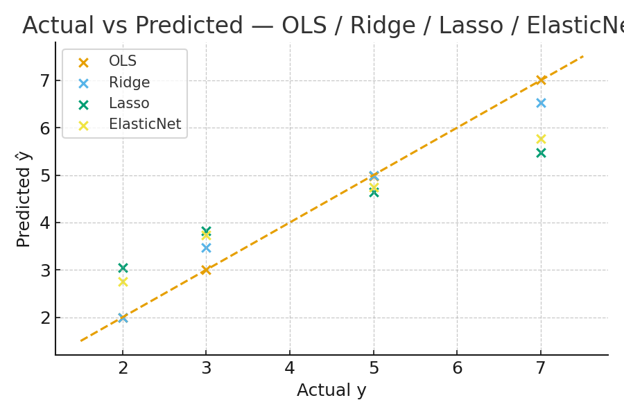
Figure: Actual vs predicted values. Points close to the diagonal indicate low bias, the model is capturing the true relationship well. -
Coefficient Path (Regularization Path)
This shows how each coefficient changes as \(\alpha\) increases. Elastic Net's path is smoother than pure Lasso, correlated features shrink together rather than one abruptly dropping to zero.
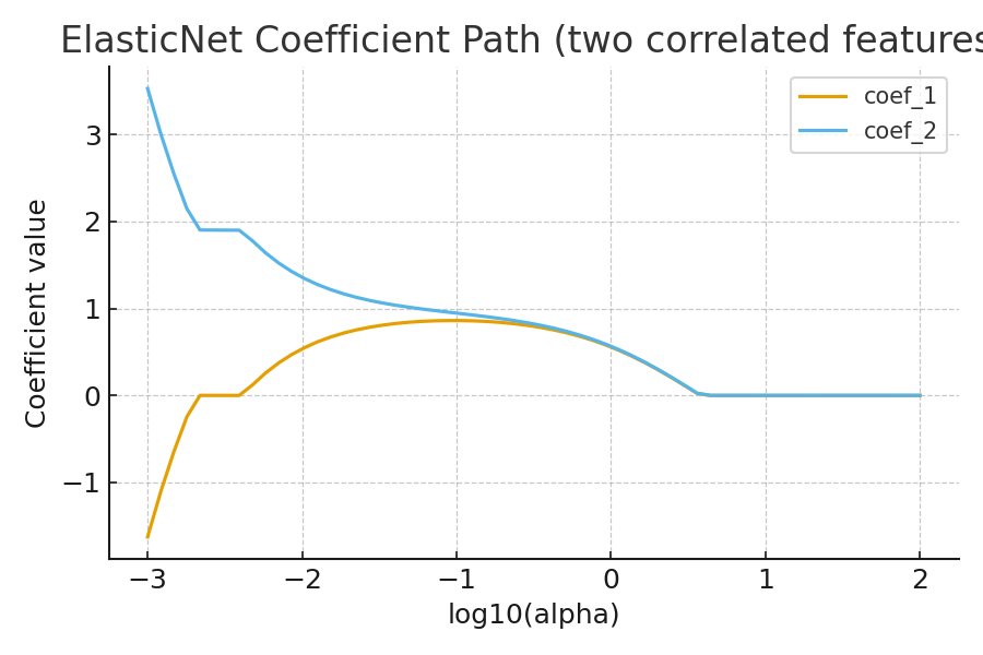
Figure: Coefficient paths as α grows. Elastic Net produces a smoother path than pure Lasso, grouping correlated predictors rather than eliminating them arbitrarily. -
Ridge vs Lasso vs Elastic Net. Coefficient Comparison
This bar chart shows the coefficients of the same model fitted with all three methods. It makes the difference immediately visible: Ridge keeps all, Lasso zeros some out, Elastic Net is in between.
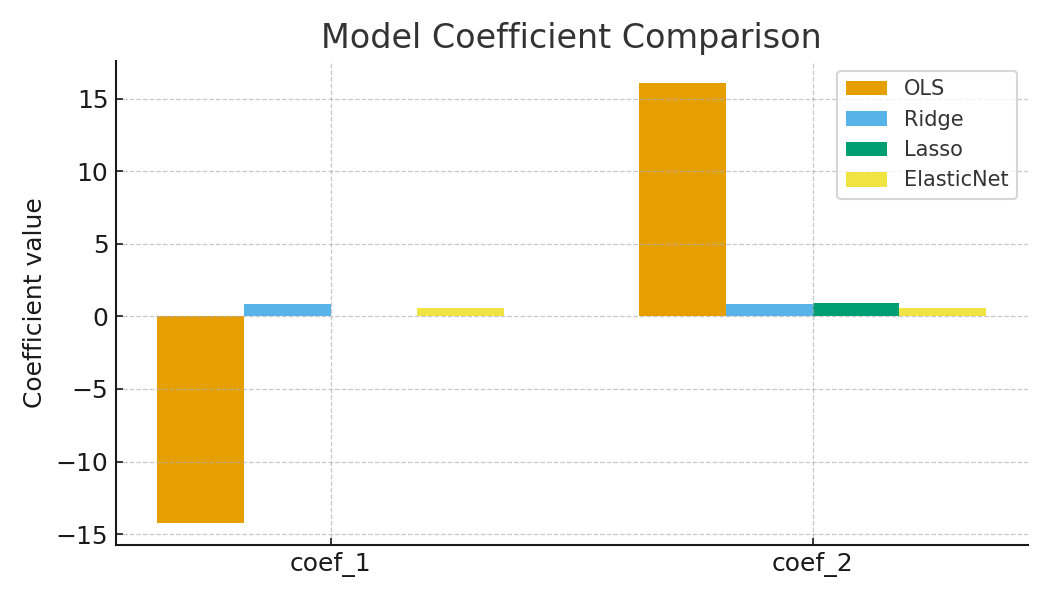
Figure: Side-by-side coefficient comparison. Ridge shrinks all, Lasso zeroes some, Elastic Net balances both behaviors. -
Residual Plot
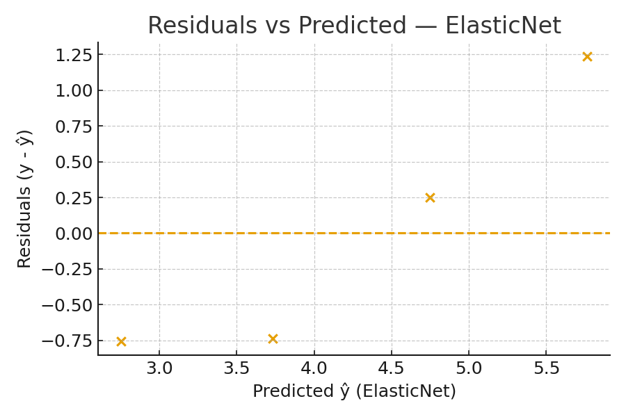
Figure: Residuals vs predicted values. Random scatter around zero indicates a well-specified model. Patterns (curves, funnels) signal missing structure. -
Elastic Net Loss Surface
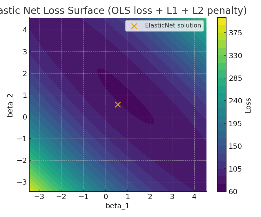
Figure: Loss surface contours showing how the Elastic Net penalty blends L1 and L2. The rounded-diamond constraint region sits visually between the pure L1 diamond and the pure L2 circle.
9. Ridge vs Lasso vs Elastic Net: When to Use Each
| Method | Penalty | Feature Selection? | Best For |
|---|---|---|---|
| Ridge | L2 (squared coefficients) | No | Correlated predictors, stability |
| Lasso | L1 (absolute values) | Yes | Many irrelevant features, sparse models |
| Elastic Net | L1 + L2 blend | Yes (grouped) | Correlated features + need for sparsity |
A practical rule of thumb:
- Start with Lasso if you have many features and expect most to be irrelevant.
- Switch to Elastic Net if Lasso behaves unstably (coefficients jumping or many correlated features).
- Use Ridge if you want to keep all features and just reduce overfitting.
10. Practical Tips
- Always standardize features before applying any regularization method. The penalty treats all coefficients equally, so features on different scales will be penalized unfairly if not scaled first.
- Tune both hyperparameters using
ElasticNetCVorGridSearchCV. Trying bothalphaandl1_ratiogives you full control over the bias-variance tradeoff. - Inspect the regularization path, a smoother path than pure Lasso indicates Elastic Net is grouping correlated features, which is usually desirable.
- Check residual plots alongside RMSE and R², a good coefficient path means nothing if the model's residuals show a systematic pattern.
11. Math Recap
The four key steps of one coordinate descent update:
- \(z = \frac{1}{n}\sum x_j(y_i - \hat y_{-j})\), partial correlation of feature \(j\) with residuals
- \(\gamma = \frac{\alpha\rho}{n}\). L1 soft-threshold
- \(S(z,\gamma) = \operatorname{sign}(z)\max(|z|-\gamma,0)\), apply soft-thresholding
- \(\beta_j = \frac{S(z,\gamma)}{1+\alpha(1-\rho)}\), apply L2 shrinkage to the surviving coefficient
Key Takeaways
- Elastic Net = Ridge (L2) + Lasso (L1), it inherits feature selection from Lasso and stability from Ridge.
- Use
alphato control overall regularization strength; usel1_ratioto control the Ridge/Lasso mix. - When predictors are correlated, Elastic Net selects them as a group rather than picking one arbitrarily (Lasso's weakness).
- Always standardize features and tune both hyperparameters with cross-validation.
References
- Zou, H., & Hastie, T. (2005). Regularization and Variable Selection via the Elastic Net. Journal of the Royal Statistical Society Series B, 67(2), 301–320.
- Scikit-learn Documentation. ElasticNet
- Hastie, T., Tibshirani, R., & Friedman, J. (2009). The Elements of Statistical Learning (2nd ed.). Springer.
- Wikipedia: Elastic Net Regularization
Related Articles